Abstract
In one of my course project, I want to know the geographical characteristics of the real estate sales of NYC. Therefore, I create a few code snippets to display the sale records on the map. In this post, you will find:
- How to get geo-coordinates based on address, i.e. address ->(longitude, latitude).
- How to display sale records on the map.
- An extension of displaying: display sale records according to their distance to a specific location.
Obtain Data and Convert Address to Geo-coordinates
- NYC real estate rolling sales data can be obtained from NYC Department of Finance.
- Upload the sale record data (.csv file) to GeoCodio to convert address to geo-coordinates.
The resulting data file includes the following columns (The columns Latitude and Longitude are added by GeoCodio):
- BOROUGH
- NEIGHBORHOOD
- BUILDING CLASS CATEGORY
- TAX CLASS AT PRESENT
- BLOCK
- LOT
- EASE-MENT
- BUILDING CLASS AT PRESENT
- Latitude
- Longitude
- ADDRESS
- APARTMENT NUMBER
- ZIP CODE
- RESIDENTIAL UNITS
- COMMERCIAL UNITS
- TOTAL UNITS
- LAND SQUARE FEET
- GROSS SQUARE FEET
- YEAR BUILT
- TAX CLASS AT TIME OF SALE
- BUILDING CLASS AT TIME OF SALE
- SALE PRICE
- SALE DATE
Take a look at the data:
import pandas as pd
import geopandas as gpd
import matplotlib.pylab as plt
import fiona
import descartes
from shapely.geometry import Point, Polygon
%matplotlib inline

# Use your own path and file name here
data = pd.read_csv('data/rollingsales_brooklyn.csv')

# Take a look at the data
data.head()| BOROUGH | NEIGHBORHOOD | BUILDING CLASS CATEGORY | TAX CLASS AT PRESENT | ... | Latitude | Longitude | ... | SALE PRICE | SALE DATE | |
|---|---|---|---|---|---|---|---|---|---|---|
| 0 | 3 | BATH BEACH | 01 ONE FAMILY DWELLINGS | 1 | ... | 40.609069 | -74.008071 | ... | 0 | 04/23/2019 |
| 1 | 3 | BATH BEACH | 01 ONE FAMILY DWELLINGS | 1 | ... | 40.609354 | -74.006997 | ... | 0 | 02/27/2019 |
| 2 | 3 | BATH BEACH | 01 ONE FAMILY DWELLINGS | 1 | ... | 40.609354 | -74.006997 | ... | 0 | 02/11/2019 |
| 3 | 3 | BATH BEACH | 01 ONE FAMILY DWELLINGS | 1 | ... | 40.607092 | -74.005414 | ... | 0 | 10/25/2018 |
| 4 | 3 | BATH BEACH | 01 ONE FAMILY DWELLINGS | 1 | ... | 40.606978 | -74.005493 | ... | 1,720,000 | 12/12/2018 |
Data Preprocessing
We notice that the conversion of address to geocoordinate, though most them fall correctly inside the boundary, some locations are still far from being correct. So before doing any analysis, we need to eliminate these outliers.
# Eliminate outliers
n = 1 # defines how many stand deviation to look for. We find n=1 is the best practice.
# Establish acceptable upper bound and lower bound for geocoordinates
lon_upper = data['Longitude'].mean() + n * data['Longitude'].std()
lon_lower = data['Longitude'].mean() - n * data['Longitude'].std()
lat_upper = data['Latitude'].mean() + n * data['Latitude'].std()
lat_lower = data['Latitude'].mean() - n * data['Latitude'].std()
# Extract those records fall within the bounds
ind = (data['Longitude'] > lon_lower) &\
 (data['Longitude'] < lon_upper) &\
 (data['Latitude'] > lat_lower) &\
 (data['Latitude'] < lat_upper)
# Copy to a a new dataframe
data2 = data.loc[ind].copy()
Displaying
In order to plot housing sale records on a map, we need a specific file called shape file. This type of file contains boundary information of a specified area using polygons. Shape file of NYC based on Zip codes could be found on NYC OpenData.
# Read shape file and remember to use your own path
tzs=gpd.read_file('data/ZIP_CODE_040114/ZIP_CODE_040114.shp')

# Transfer tzs to 'epsg:4326' coordinates
# 'epsg:4326' is the type of geolocation encoding method we used in our data set
tzs = tzs.to_crs({'init':'epsg:4326'})

# Merge tzs with our housing data
geometry = [Point(xy) for xy in zip(data2['Longitude'],data2['Latitude'])]
crs = {'init':'epsg:4326'}
geo_df = gpd.GeoDataFrame(data2, crs = crs, geometry = geometry)

# Take a look at what we have now
geo_df.head()| BOROUGH | NEIGHBORHOOD | ... | Latitude | Longitude | ... | SALE PRICE | SALE DATE | geometry | |
|---|---|---|---|---|---|---|---|---|---|
| 0 | 3 | BATH BEACH | ... | 40.609069 | -74.008071 | ... | 0 | 04/23/2019 | POINT (-74.00807 40.60907) |
| 1 | 3 | BATH BEACH | ... | 40.609354 | -74.006997 | ... | 0 | 02/27/2019 | POINT (-74.00700 40.60935) |
| 2 | 3 | BATH BEACH | ... | 40.609354 | -74.006997 | ... | 0 | 02/11/2019 | POINT (-74.00700 40.60935) |
| 3 | 3 | BATH BEACH | ... | 40.607092 | -74.005414 | ... | 0 | 10/25/2018 | POINT (-74.00541 40.60709) |
| 4 | 3 | BATH BEACH | ... | 40.606978 | -74.005493 | ... | 1,720,000 | 12/12/2018 | POINT (-74.00549 40.60698) |
Notice the last column “geometry”, which tells where the point will be on a plot.
Alright, let’s see where these sales happened.
# Take a look at the housing sales' location.
fig, ax = plt.subplots(figsize = (12, 12))
tzs.plot(ax = ax, alpha = 1, color = '#cacfd9') # pick the color you want
ax = geo_df.plot(ax = ax, color = '#db7846', marker = 'o', markersize = 0.05)
ax.set_xlabel("Latitude")
ax.set_ylabel("Longitude")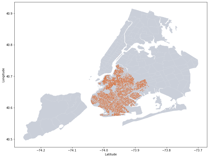 |
|---|
| Fig 1. Real estate sale records of Brooklyn, NY, from 10/01/2018 to 09/30/2019 |
We see that the data well spread across Brooklyn. We can also observe several blank area in the middle, they are either parks, cemetery, or golf center, according to Google map.
Displaying Based on Distance to a Specific Point
Now, considering that some institutions or commercial centers may have significant influence to the local housing market, we perhaps want to correlate the housing price with respect to their distances to these places.
Let’s choose the Tandon Engineering School of NYU for example (This is where I am currently studying. You can choose any places you like :)).
# Just like what we had done before, we formulate a geo file for Tandon here.
# Geocoordinate can be easily find through Google map.
c_tandon = pd.DataFrame([[40.693579, -73.985701]],columns = ['Latitude','Longitude'])
geometry_tandon = [Point(xy) for xy in zip(c_tandon['Longitude'],c_tandon['Latitude'])]
geo_tandon_df = gpd.GeoDataFrame(c_tandon, crs = crs, geometry = geometry_tandon)
ax.set_xlabel("Latitude")
ax.set_ylabel("Longitude")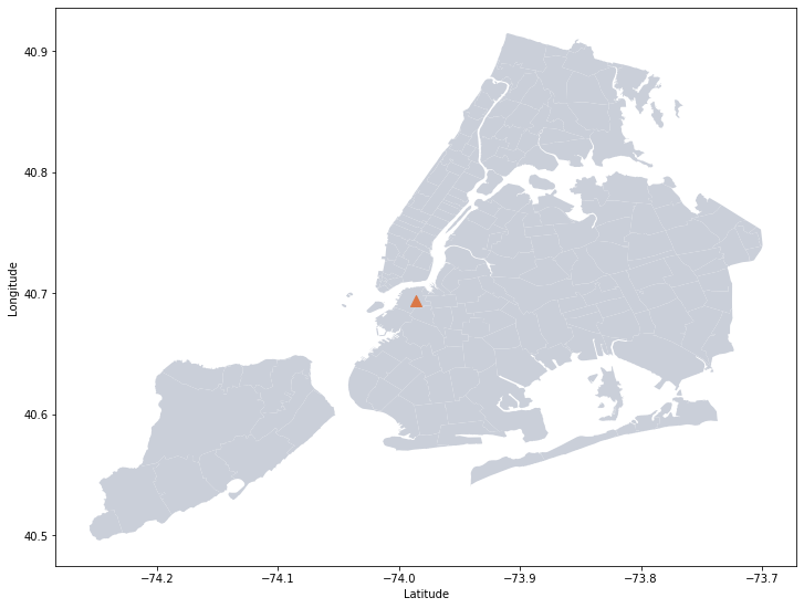 |
|---|
| Fig 2. Tandon School of Engineering, Brooklyn, NY |
Now, we want to calculate how far thoes sales are away from Tandon School.
lon_dis = 52.8 # 1 unit of longitude = 52.8 miles (around NYC's latitude)
lat_dis = 69.0 # 1 unit of latitude = 69.0 miles (almost a constant everywhere)

# calculate straight line distance
dis_lon = (geo_df['Longitude'] - c_tandon['Longitude'][0]) * lon_dis
dis_lat = (geo_df['Latitude'] - c_tandon['Latitude'][0]) * lat_dis
geo_df['dis_to_Tandon'] = (dis_lon ** 2 + dis_lat ** 2) ** 0.5
Then, let’s group these sales according to their distance to Tandon School.
# seperate into 6 groups, you can do any other numbers
dis_group = [0, 0.5, 1, 2, 5, 10, 20]
legend = list()

fig, ax = plt.subplots(figsize = (12, 12))
tzs.plot(ax = ax, alpha = 1, color = '#cacfd9')

for i in range(0, len(dis_group) - 1):
    cond = (geo_df['dis_to_Tandon']>dis_group[i]) & (geo_df['dis_to_Tandon'] < dis_group[i + 1])
    geo_df[cond].plot(ax = ax, marker = 'o', markersize = 0.05)
    legend.append(str(dis_group[i]) + 'mi < d < ' + str(dis_group[i + 1]) + 'mi')

plt.legend(legend, markerscale = 20)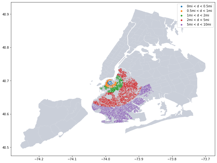 |
|---|
| Fig 3. Grouping real estate sale records according to their distance to Tandon School |
Closing Notes
The key tools/files used to perform the task are:
- Geo-API, e.g. GeoCodio, to convert address to geo-coordinates.
- Python package geopandas, which converts geo-coordinates to POINT objects (to be displayed on a map).
- Shapefile, which is a kind of map consists of polygon areas. POINTs are to be displayed on them.