Abstract
In one of my course projects, we need to analyze the seasonal pattern of Citibike riderships. I find taking some notes on how to handle Citibike data will be helpful for future reference.
This blog will demonstrate the following items:
- Read Citibike trip history data.
- Aggregate trip history data by month.
- Display trip history data based on user type, gender, and age group.
Citibike provides a comprehensive list of trip history data in their homepage. It includes the following columns:
- Trip Duration (seconds)
- Start Time and Date
- Stop Time and Date
- Start Station Name
- End Station Name
- Station ID
- Station Lat/Long
- Bike ID
- User Type (Customer = 24-hour pass or 3-day pass user; Subscriber = Annual Member)
- Gender (Zero=unknown; 1=male; 2=female)
- Year of Birth
Read Data
Let’s read a sample of the data to see how it looks like. Suppose we are interested in the data between 2016 - 2019. We have the data files downloaded and stored in the path ‘/data’.
import pandas as pd
import numpy as np
import matplotlib.pylab as plt
from datetime import datetime

y_ind = ['2016','2017','2018','2019'] # list of years interested
m_ind = list()
for i in range(1,13):
    m_ind.append(str(i)) # list of months

# take a look at a data sample
data = pd.read_csv("data/201710-citibike-tripdata.csv")
data.head(5)| tripduration | starttime | stoptime | start station id | start station name | start station latitude | ... | usertype | birth year | gender | |
|---|---|---|---|---|---|---|---|---|---|---|
| 0 | 457 | 2017-10-01 00:00:00 | 2017-10-01 00:07:38 | 479 | 9 Ave & W 45 St | 40.760193 | ... | Subscriber | 1985.0 | 1 |
| 1 | 6462 | 2017-10-01 00:00:20 | 2017-10-01 01:48:03 | 279 | Peck Slip & Front St | 40.707873 | ... | Customer | NaN | 0 |
| 2 | 761 | 2017-10-01 00:00:27 | 2017-10-01 00:13:09 | 504 | 1 Ave & E 16 St | 40.732219 | ... | Subscriber | 1992.0 | 1 |
| 3 | 1193 | 2017-10-01 00:00:29 | 2017-10-01 00:20:22 | 3236 | W 42 St & Dyer Ave | 40.758985 | ... | Customer | 1992.0 | 2 |
| 4 | 2772 | 2017-10-01 00:00:32 | 2017-10-01 00:46:44 | 2006 | Central Park S & 6 Ave | 40.765909 | ... | Customer | NaN | 0 |
Pre-processing
Let’s say we are interested in a month-by-month pattern. For each month, the data file could be at the size of 100M. Therefore, we want to preprocess (i.e. extract and aggregate) the data before doing anything else. Say we are interested in the information about user types, gender, and age.
# assume we want to analyze the behavior of different user types, genders, and age groups
# initialize empty dataframes for each type of analysis
data_user = pd.DataFrame()
data_gender = pd.DataFrame()
data_age = pd.DataFrame()
Then, we will loop over all the data files and extract related information (Citibike changes the format or the column titles along the way, so we need to pay special attention to these change. You can read the accomodations in the following codes).
# Loop over all years and months.
# I suggest to start with 1 datafile, e.g. y_ind = [2019], m_ind = [1], for the test run.
# The entire 4 years' data takes me 20min to run with a 16G RAM and a good CPU.
for y in y_ind:
    for m in m_ind:
        # If month is '1-9', turn it to '01-09' for consistency.
        if len(m) == 1:
            m_temp = "0" + m
        else:
            m_temp = m

        # Try to load data, when finished, print
        try:
            data1 = pd.read_csv("data/" + y + m_temp + "-citibike-tripdata.csv")
        except:
            print('Finish reading all the data')

        # Print some notes to know how many files we have loaded
        print("---------")
        print(y + m_temp + "-citibike-tripdata.csv")

        # Preprocessing step 1: uniform column names
        # data between 2016-10 and 2017-02 has different column names from other time.
        # We want to change them to uniformed names
        try:
            data1['starttime'] # the column name is either 'startime' or 'Start Time'
        except:
            data1.rename(columns={u'Start Time' : 'starttime',\
                     u'Bike ID' : 'bikeid', \
                     u'User Type' : 'usertype',\
                     u'Birth Year' : 'birth year',\
                     u'Gender' : 'gender',\
                      u'Trip Duration' : 'tripduration'}, inplace=True)
            print("Note: Column name is corrected")

        # Preprocessing step 2: remove NaN values
        ind = (pd.notna(data1['birth year'])) &\
		(pd.notna(data1['gender'])) &\
		(pd.notna(data1['usertype']))

        data_temp = data1.loc[ind].copy()
        s = pd.Series(range(0,len(data_temp.index))) # reorganize index
        data_temp.set_index([s],inplace = True)

        # Preprocessing step 3: Convert time str to datetime object
        # Citibike data file has the following 4 types of date str, e.g.:
		# 2019-01-31, 1/3/2019, 1/31/2019, 10/31/2019
		# We need to test each one until we get a correct result
        try:
            time = datetime.strptime(data_temp['starttime'][0][0:10], '%Y-%m-%d')
        except:
            try:
                time = datetime.strptime(data_temp['starttime'][0][0:8], '%m/%d/%Y')
            except:
                try:
                    time = datetime.strptime(data_temp['starttime'][0][0:9], '%m/%d/%Y')
                except:
                    time = datetime.strptime(data_temp['starttime'][0][0:10], '%m/%d/%Y')

        # Now we have finished data cleaning, let's start to aggregate the data to each type

        # 1. Generate Usertype data:
		# Columns: all, subscriber (sub), and customer (cus)
        data_temp_user = pd.DataFrame()
        data_temp_user['time'] = pd.Series(time)
        # set index to be 2 columns and count along 'usertype'
        count1 = data_temp.set_index(['usertype','tripduration']).count(level = 'usertype').bikeid
        data_temp_user['count_all'] = pd.Series(sum(count1))
        data_temp_user['count_sub'] = pd.Series(count1.Subscriber)
        # for some months, only subscribers ride Citibike
        try:
            data_temp_user['count_cus'] = pd.Series(count1.Customer)
        except:
            data_temp_user['count_cus'] = pd.Series(0)
            print('Note: There is no casual customer for ' + y + '-' + m_temp)
        # add monthly data to a predefined dataframe
        data_user = data_user.append(data_temp_user)

        # 2. generate Gender data
		# Columns: all, male (m), female (f), and undisclosed (u)
        data_temp_gender = pd.DataFrame()
        data_temp_gender['time'] = pd.Series(time)
        count2 = data_temp.set_index(['gender','tripduration']).count(level = 'gender').bikeid
        data_temp_gender['count_all'] = pd.Series(sum(count2))
        data_temp_gender['count_m'] = pd.Series(count2[1]) # male
        data_temp_gender['count_f'] = pd.Series(count2[2]) # female
        data_temp_gender['count_u'] = pd.Series(count2[0]) # unknown
        data_gender = data_gender.append(data_temp_gender)

        # 3. generate Age data
		# Columns: according to the age group specified below
        data_temp_age = pd.DataFrame()
        data_temp_age['time'] = pd.Series(time)
        data_temp['age'] = int(y) - data_temp['birth year'] # calculate age
        # split age groups. Only age over 16 is allowed to use Citibike
        age_group = [16,18,22,30,40,50,60,70,max(data_temp.age)]
        # use 'groupby' and 'cut' method to count over age groups
        count3 = data_temp.groupby(pd.cut(data_temp.age, age_group)).count().bikeid
        data_temp_age['count_all'] = pd.Series(sum(count3))
        # assign result to each age group
        for i in range(0,len(age_group) - 1):
            data_temp_age['count_g' + str(i + 1)] = pd.Series(count3[i])
        data_age = data_age.append(data_temp_age)
Now let’s take a look of what we have obtained:
s1 = pd.Series(range(0,len(data_user.index)))
data_user.set_index([s1],inplace = True) # assign index
data_user.head()| time | count_all | count_sub | count_cus | |
|---|---|---|---|---|
| 0 | 2016-01-01 | 484933 | 484933 | 0 |
| 1 | 2016-02-01 | 531048 | 531048 | 0 |
| 2 | 2016-03-01 | 826678 | 826678 | 0 |
| 3 | 2016-04-01 | 882679 | 882679 | 0 |
| 4 | 2016-05-01 | 1035959 | 1035959 | 0 |
s2 = pd.Series(range(0,len(data_gender.index)))
data_gender.set_index([s2],inplace = True)
data_gender.head()| time | count_all | count_m | count_f | count_u | |
|---|---|---|---|---|---|
| 0 | 2016-01-01 | 484933 | 379312 | 104457 | 1164 |
| 1 | 2016-02-01 | 531048 | 417215 | 112587 | 1246 |
| 2 | 2016-03-01 | 826678 | 634214 | 190551 | 1913 |
| 3 | 2016-04-01 | 882679 | 674127 | 206510 | 2042 |
| 4 | 2016-05-01 | 1035959 | 783687 | 249831 | 2441 |
s3 = pd.Series(range(0,len(data_age.index)))
data_age.set_index([s3],inplace = True)
data_age.head()| time | count_all | count_g1 | count_g2 | count_g3 | ... | count_g7 | count_g8 | |
|---|---|---|---|---|---|---|---|---|
| 0 | 2016-01-01 | 484932 | 1707 | 6548 | 109880 | ... | 22729 | 2973 |
| 1 | 2016-02-01 | 531025 | 1875 | 12614 | 125913 | ... | 24657 | 3308 |
| 2 | 2016-03-01 | 826631 | 2780 | 18494 | 208283 | ... | 37196 | 5162 |
| 3 | 2016-04-01 | 882548 | 2822 | 20496 | 235703 | ... | 37163 | 5271 |
| 4 | 2016-05-01 | 1035719 | 3730 | 21318 | 280539 | ... | 41444 | 5754 |
Great! After a bunch of work, we successfully extract monthly aggregated data for each scenario. We want to save them to our local disk, then next time we want to use them, we don’t need to go over this time-consuming procedure again:
data_user.to_csv('data_usertype.csv')
data_gender.to_csv('data_gender.csv')
data_age.to_csv('data_age.csv')
Visualization
Now, its time to have some good plots.
First of all, let’s see how user type looks like.
plt.figure(figsize=(12,5))
plt.plot(data_gender['time'], data_gender['count_all'],'>-')
plt.plot(data_gender['time'], data_gender['count_m'],'o-')
plt.plot(data_gender['time'], data_gender['count_f'],'*-')
plt.plot(data_gender['time'], data_gender['count_u'],'^-')
plt.ylabel('Ridership')
plt.xlabel('Time')
plt.legend(['all','male','female','unknown'])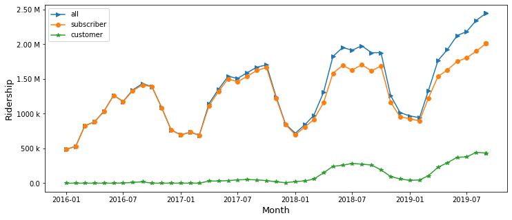 |
|---|
| Fig 1. How ridership splited among subscribers and customers |
We notice a clear pattern of seasonal dynamics. The ridership peaks in Sep or Oct, and reaches its valley in winter.
A another fact is that subscribers have a dominant share of ridership in Citibike, but we can also see an increasing trend of customer ridership during recent years.
Then, what about genders?
plt.figure(figsize=(12,5))
plt.plot(data_user['time'], data_user['count_all'],'>-')
plt.plot(data_user['time'], data_user['count_sub'],'o-')
plt.plot(data_user['time'], data_user['count_cus'],'*-')
plt.ylabel('Ridership')
plt.xlabel('Time')
plt.legend(['all','subscriber','customer'])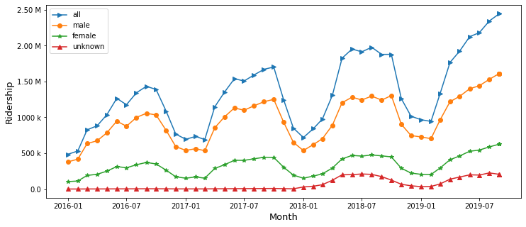 |
|---|
| Fig 2. How ridership splited among genders |
Suprisingly, though NYC has a larger share of females, the ridership is performed more by males. Huh, funny. Is it because males prefer biking than females?
Also, started from 2018, more users reported their gender to be unknown. This could be explained by thinking that people have been getting more awared of pravicy protection in using apps, or simply, Citibike provided a 3rd selection of genders since 2018.
Finally, how does age influences ridership?
plt.figure(figsize=(12,5))
legend = list()
for i in range(0,len(age_group) - 1):
    plt.plot(data_age['time'], data_age['count_g' + str(i + 1)],'o-')
    legend.append(str(age_group[i]) + '~' + str(age_group[i + 1]))
legend[-1] = '70+'
plt.legend(legend)
plt.ylabel('Ridership')
plt.xlabel('Time')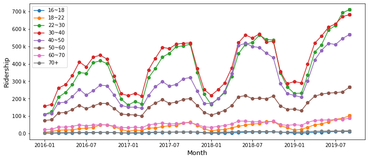 |
|---|
| Fig 3. How ridership splited among age groups |
Clearly, working age people use Citibike the most.
Closing Notes
Citibike provides a good dataset for research purposes. This blog is intended to show how to process a large amount of CItibike data files and extract useful information.